

How is linearity checked in EIS with Lissajous plots and the Fourier transform? (CVSim example)
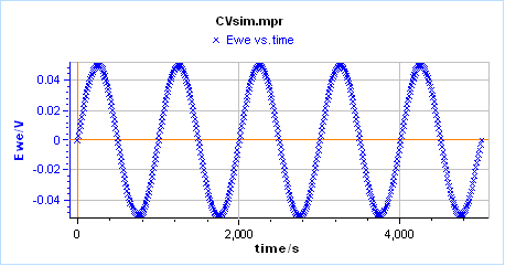
Using the free-access CVSim simulator in EC-Lab, 10 mV and 50 mV sine perturbations are applied to a simple redox reaction (E mechanism); linear and non-linear responses are compared in the time, Lissajous and frequency domains.
Key points
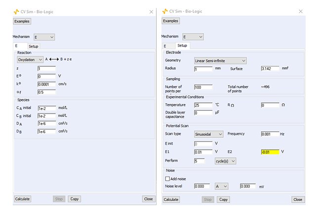
- Simulation: E mechanism, both redox species initially in solution (10 mM), k° = 10⁻⁴ cm/s, αf = 0.5, D = 10⁻⁶ cm²/s, 1 mHz sine excitation.
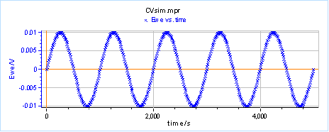
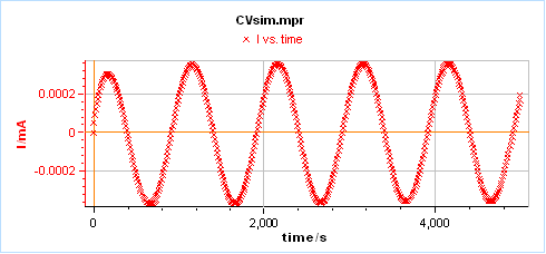
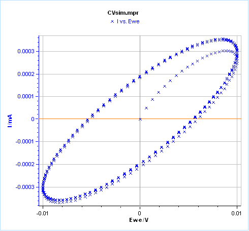
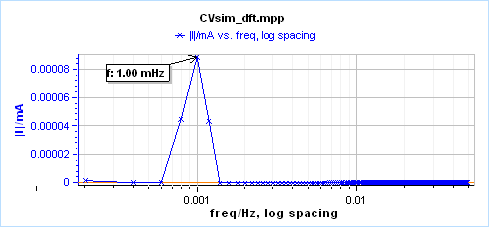
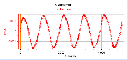
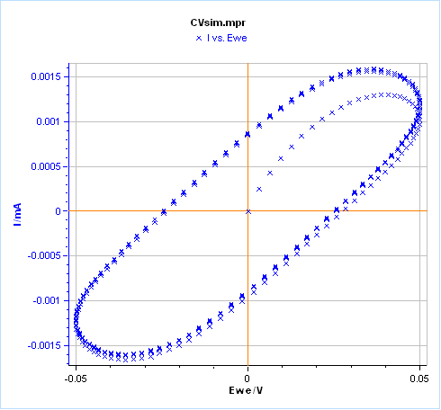
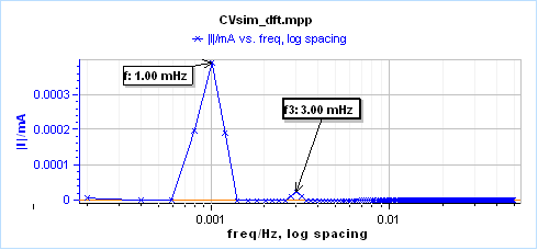
- At 10 mV the current is a pure sine after the first period, the Lissajous plot (I vs E) is an ellipse and the Fourier transform shows a single line at 1 mHz: the system behaves linearly.
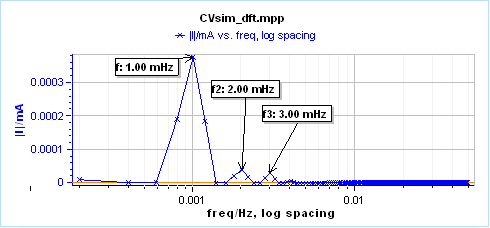
- At 50 mV the current response is distorted, the Lissajous plot departs from an ellipse and a third harmonic appears at 3 mHz in the Fourier spectrum, definite proof of non-linearity.
- Only the third harmonic appears because the symmetry factor is αf = 0.5; with αf = 0.1 a second harmonic appears at 2 mHz as well. More harmonics appear as the amplitude increases.
- The Fourier transform is far more sensitive and quantitative than the shape-based, qualitative Lissajous method. The THD, NSD and NSR indicators in EC-Lab are calculated from this discrete Fourier transform.
Figures
Images: Bio-Logic Science Instruments; taken from the source article.
Related application notes
- Is my system linear? How does the excitation amplitude distort the EIS result? Battery AN9
- Which parameters affect the THD value, and how does it compare with other linearity tests? Corrosion AN65
- What do the EIS quality indicators THD, NSD and NSR tell us? Corrosion AN64
- CV Sim 1: How does the scan rate affect the voltammogram of a simple redox reaction? Kinetics AN41-1
Related curriculum module: Electrochemical Impedance Spectroscopy (EIS)
Source: Bio-Logic Learning Center, “CVSim as a learning tool III: Linearity in EIS” · Source updated: November 18, 2024
Copyright of the images and the original text belongs to Bio-Logic SAS.
Copyright of the images and the original text belongs to Bio-Logic SAS.