
Bio-LogicBio-Logic Science Instruments Authorized Distributor for Türkiye
+90 (312) 437 40 77  ·  [email protected]
TR/EN
Get a Quote
Popular topics · Getting started with EIS

What is EIS, how is it represented and how is it interpreted?

The definition of electrochemical impedance spectroscopy, Nyquist and Bode representations, the linearity and stationarity requirements, choosing the critical measurement parameters and interpretation with equivalent circuits: a comprehensive guide to getting started with EIS.

Key points

  • DC techniques (chronoamperometry, chronopotentiometry, LSV, CV) study the response of a system as a function of time; EIS studies the response to a small sine perturbation as a function of frequency. A sweep from MHz to µHz covers processes lasting from below a microsecond to hundreds of hours in a single measurement.
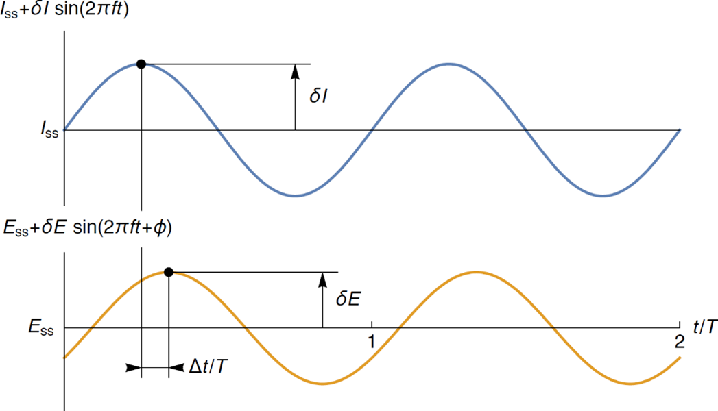
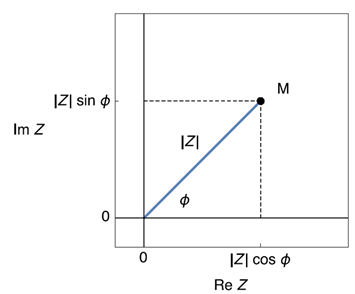
  • In a linear time-invariant (LTI) system the response is a phase-shifted sine at the same frequency: |Z| = δE/δI and φ = 2πΔt/T. Modulus and phase are the polar representation, real and imaginary parts the Cartesian one.
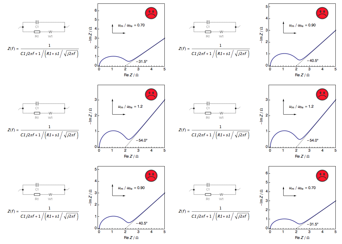
  • The Nyquist plot (−Im Z vs Re Z) shows frequency implicitly, the Bode plot (|Z| and φ vs f) explicitly. Nyquist plots must always be drawn with equal axis scales (orthonormal); otherwise the 45° Warburg line and semicircles are misread.
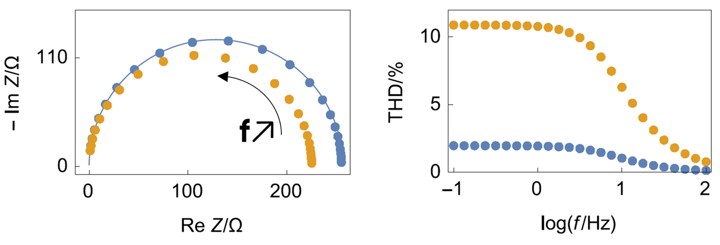
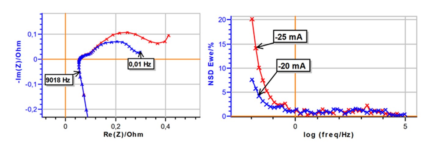
  • Electrochemical systems are non-linear by nature; linearity is obtained with a small enough amplitude and checked quantitatively with THD (5% is a common threshold). Stationarity is checked with NSD; in the example, data below about 0.1 Hz on an 18650 LFP cell are affected by the discharge current.
  • The upper frequency is chosen to reach the series resistance (typically 1 - 10 kHz); in low-impedance systems inductive behaviour appears at high frequency and must be accounted for in the fit. Below 1 Hz, multisine shortens the measurement; the wait time (Pw) and drift correction improve low-frequency data.
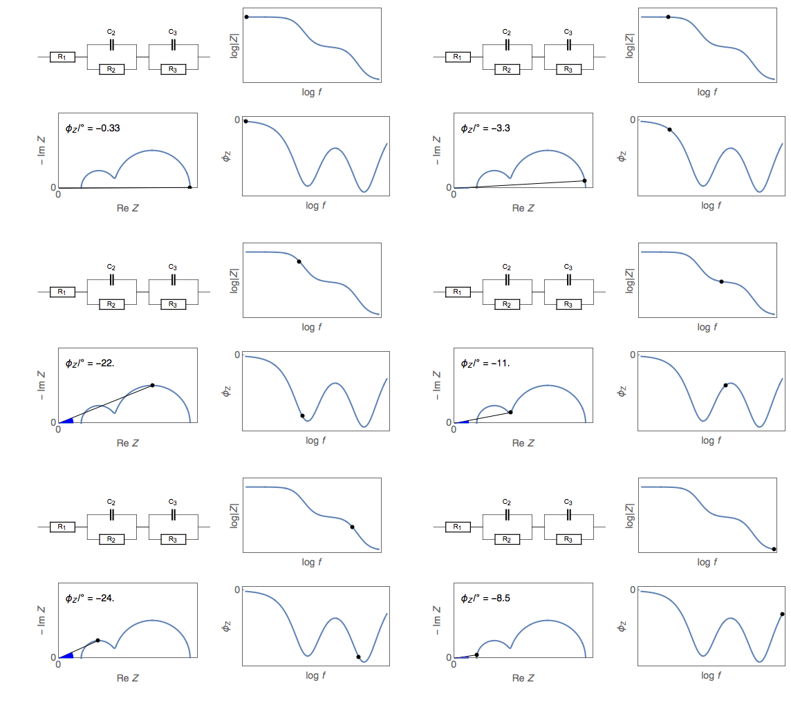
  • Interpretation uses an equivalent circuit fitted with ZFit. The figures show the basic circuits and the processes they represent. A full battery has two electrode interfaces, so the faradaic part appears twice; the double-layer capacitance can be represented by a constant phase element (CPE, Q) instead of C.

Figures
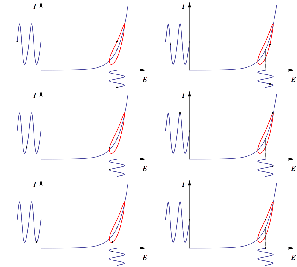
A small sine excitation on a non-linear I-E curve: as amplitude grows the Lissajous curve stops being an ellipse.
Figure 1. A small sine excitation on a non-linear I-E curve: as amplitude grows the Lissajous curve stops being an ellipse.
A linear time-invariant (LTI) system: a sine input gives a phase-shifted sine output at the same frequency.
Figure 2. A linear time-invariant (LTI) system: a sine input gives a phase-shifted sine output at the same frequency.
Current and potential sines: |Z| = δE/δI, phase φ = 2πΔt/T.
Figure 3. Current and potential sines: |Z| = δE/δI, phase φ = 2πΔt/T.
Polar and Cartesian representation of impedance: Re Z = |Z| cos φ, Im Z = |Z| sin φ.
Figure 4. Polar and Cartesian representation of impedance: Re Z = |Z| cos φ, Im Z = |Z| sin φ.
The same data in Nyquist and Bode plots: each Nyquist point corresponds to one frequency.
Figure 5. The same data in Nyquist and Bode plots: each Nyquist point corresponds to one frequency.
If the axis scales are unequal the 45° Warburg slope looks wrong; Nyquist plots must be drawn orthonormal.
Figure 6. If the axis scales are unequal the 45° Warburg slope looks wrong; Nyquist plots must be drawn orthonormal.
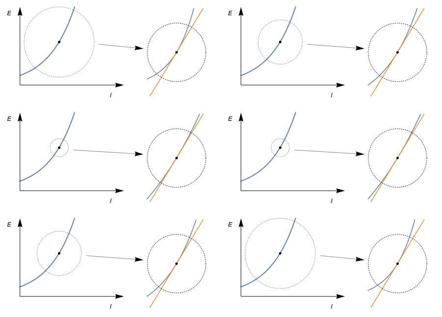
Principle of linearity: a small enough part of the curve approximates a straight line; the excitation must stay in that region.
Figure 7. Principle of linearity: a small enough part of the curve approximates a straight line; the excitation must stay in that region.
At large amplitude (orange) the arc shrinks and THD exceeds 5%; at a suitable amplitude (blue) THD is low.
Figure 8. At large amplitude (orange) the arc shrinks and THD exceeds 5%; at a suitable amplitude (blue) THD is low.
Nyquist and NSD of an 18650 LFP cell at two discharge currents (-20 and -25 mA): below about 0.1 Hz the data lose stationarity.
Figure 9. Nyquist and NSD of an 18650 LFP cell at two discharge currents (-20 and -25 mA): below about 0.1 Hz the data lose stationarity.
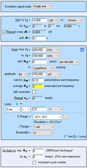
EC-Lab GEIS settings window: frequency range, points per decade, amplitude, wait (Pw) and average (Na).
Figure 10. EC-Lab GEIS settings window: frequency range, points per decade, amplitude, wait (Pw) and average (Na).
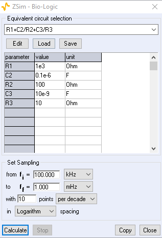
ZSim: impedance simulation from an equivalent circuit and its parameters.
Figure 11. ZSim: impedance simulation from an equivalent circuit and its parameters.
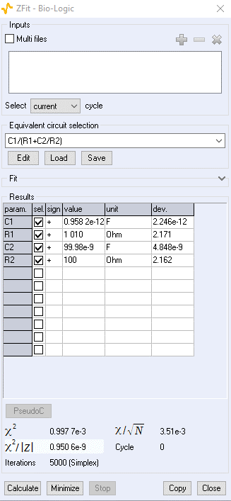
ZFit results window: parameter values, standard errors and goodness of fit via χ².
Figure 12. ZFit results window: parameter values, standard errors and goodness of fit via χ².
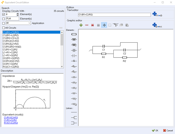
EC-Lab equivalent circuit editor: circuit library, text and graphic editing, impedance expression.
Figure 13. EC-Lab equivalent circuit editor: circuit library, text and graphic editing, impedance expression.
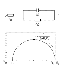
R1 + C2/R2: charge transfer without mass-transport limitation (Butler-Volmer, Tafel-type corrosion); apex frequency 1/(2πR2C2).
Figure 14. R1 + C2/R2: charge transfer without mass-transport limitation (Butler-Volmer, Tafel-type corrosion); apex frequency 1/(2πR2C2).
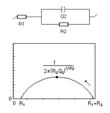
R1 + Q2/R2: a depressed semicircle when a CPE replaces the double layer.
Figure 15. R1 + Q2/R2: a depressed semicircle when a CPE replaces the double layer.
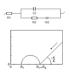
R1 + C2/(R2 + W2): charge transfer and semi-infinite diffusion; 45° Warburg line at low frequency.
Figure 16. R1 + C2/(R2 + W2): charge transfer and semi-infinite diffusion; 45° Warburg line at low frequency.
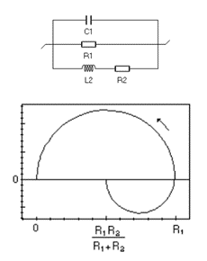
C1/R1/(L2 + R2): charge transfer and adsorption (Volmer-Heyrovský); low-frequency inductive loop in acidic corrosion and electrocatalysis.
Figure 17. C1/R1/(L2 + R2): charge transfer and adsorption (Volmer-Heyrovský); low-frequency inductive loop in acidic corrosion and electrocatalysis.
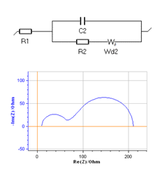
R1 + C2/(R2 + Wd2): charge transfer and convection-diffusion; a second arc for rotating disk electrodes, fuel cells and flow batteries.
Figure 18. R1 + C2/(R2 + Wd2): charge transfer and convection-diffusion; a second arc for rotating disk electrodes, fuel cells and flow batteries.
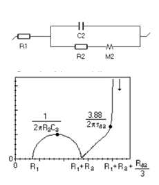
R1 + C2/(R2 + M2): charge transfer and restricted diffusion (insertion reaction); vertical capacitive branch in Li-ion batteries, Re Z limit R1 + R2 + Rd/3.
Figure 19. R1 + C2/(R2 + M2): charge transfer and restricted diffusion (insertion reaction); vertical capacitive branch in Li-ion batteries, Re Z limit R1 + R2 + Rd/3.

Images: Bio-Logic Science Instruments; taken from the source article.

Videos

Related application notes

Related curriculum module: Electrochemical Impedance Spectroscopy (EIS)

Source: Bio-Logic Learning Center, “What is Electrochemical Impedance Spectroscopy (EIS)? Electrochemistry Basics Series” · Source updated: August 20, 2026
Copyright of the images and the original text belongs to Bio-Logic SAS.

All popular topics

Would you like to set up this measurement in your laboratory?

Contact our technical team for the suitable instrument, cell and software configuration.

Quotation and technical consulting