

How is EIS data from a time-variant system checked and corrected?
A low-frequency measurement is like a long-exposure photograph: if the system changes during the measurement, the data blur. The difference between steady state and time invariance, diagnosis with NSD and correction with the EC-Lab Z Inst tool.
Key points
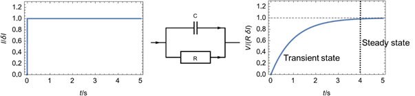
- For valid EIS the system must be linear, stable, causal and stationary. Stationarity has two parts: steady state (transients have decayed) and time invariance (the parameters defining the transfer function stay constant).
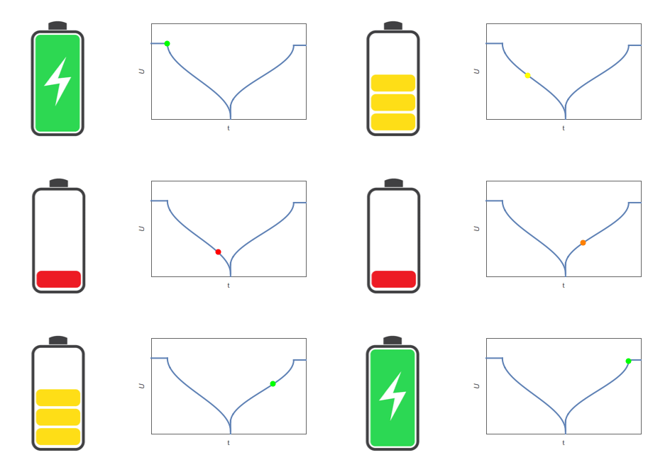
- Examples: on a corroding electrode the polarisation resistance changes with corrosion or passivation; in a discharging battery the charge-transfer and diffusion resistances change continuously.
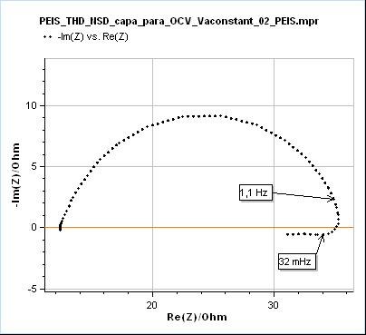
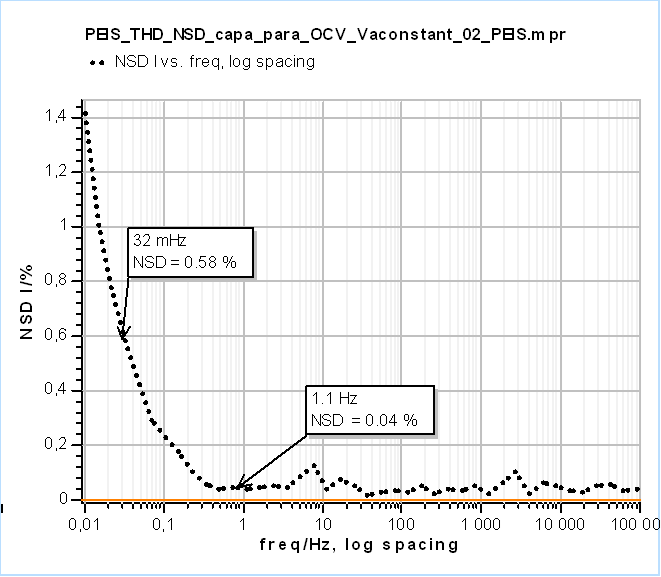
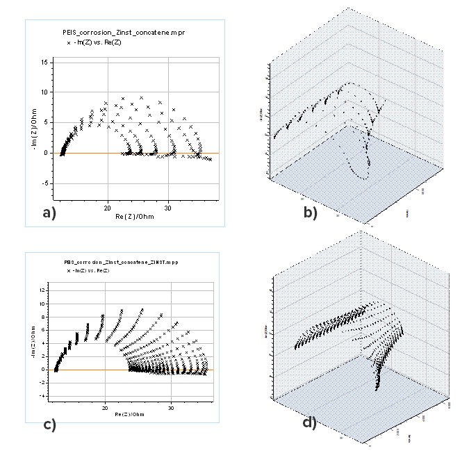
- The effect is usually seen at low frequencies, because the changes are slower than high frequencies such as 1 MHz - 10 Hz. In the example NSD rises from 1.1 Hz; although it is only 0.58% at 32 mHz, the low-frequency data are clearly distorted. Even small NSD values can be significant.
- Correction: the EC-Lab Z Inst tool applies the method of Stoynov and Savova. Successive spectra are arranged against time, points at the same frequency are connected and interpolated to form an impedance surface, and cross-sections at chosen instants give instantaneous spectra free of time variance.
- The corrected spectra are fitted with ZFit to obtain Cdl, Rct and Rp, the low-frequency limit. The low-frequency inductive part in acidic medium shows that proton reduction involves an adsorption step.
Figures
Images: Bio-Logic Science Instruments; taken from the source article.
Related application notes
- Why is EIS misinterpreted on time-varying systems? Corrosion AN55
- How is EIS corrected when the system drifts during the measurement? Battery AN17
- How is a non-stationary EIS measurement detected and corrected? (Corrosion example) Corrosion AN69-1
- How is a non-stationary EIS measurement corrected? (Battery cell example) Battery AN69-2
- What do the EIS quality indicators THD, NSD and NSR tell us? Corrosion AN64
Related curriculum module: Electrochemical Impedance Spectroscopy (EIS)
Source: Bio-Logic Learning Center, “How to check and correct the time variance of your system under EIS measurements” · Source updated: April 13, 2026
Copyright of the images and the original text belongs to Bio-Logic SAS.
Copyright of the images and the original text belongs to Bio-Logic SAS.